TESS example#

This notebook walks through a few examples that show how to use TRICERATOPS. The examples below show:

How to apply TRICERATOPS on a star observed in a \(\textbf{single}\) \({\it TESS}\) sector \(\textbf{without}\) follow up data.
How to apply TRICERATOPS on a star observed in a \(\textbf{single}\) \({\it TESS}\) sector \(\textbf{with}\) follow up data.
How to apply TRICERATOPS on a star observed in \(\textbf{multiple}\) \({\it TESS}\) sectors \(\textbf{without}\) follow up data.

[1]:

import numpy as np
import pandas as pd
import time
from lightkurve import TessLightCurve
import matplotlib.pyplot as plt
%matplotlib inline

import triceratops.triceratops as tr

Example #1#

First, let’s apply the tool on TOI 465.01 (aka TIC 270380593.01, aka WASP-156b), which was observed with a 2 minute cadence in sector 4.

Begin by defining the target star object with the target(ID, sectors) class. The arguments for this class are ID (the TIC ID of the star) and sectors (the sectors in which the star was observed). ID should be an integer and sectors should be a numpy array.

[2]:

ID = 270380593
sectors = np.array([4])
target = tr.target(ID=ID, sectors=sectors)

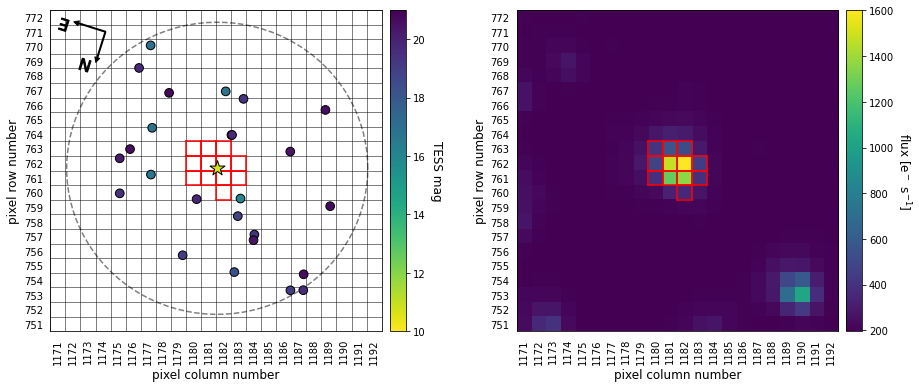
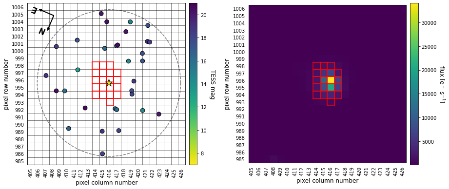
Next, let’s define the aperture used to extract the light curve, plot an image of the field, and display a table of nearby stars.

The aperture should be a 2D numpy array with the formal [[col#, row#], [col#, row#], [col#, row#], ...], where where each [col#, row#] is the column and row number of the pixel.

An image of the field can be plotted with the .plot_field(sector, ap_pixels) method. This method takes as optional arguments sector (the image sector you would like to plot) and ap_pixels (the aperture we just defined).

We can display a table of the stars in the image with the .stars attribute. This table contains the separation and position angle of each star from the target star, so that each can be identified in the plot. Note that the scale of a TESS pixel is about 20 arcseconds.

[3]:

ap = np.array([ [1180, 763], [1181, 763], [1182, 763],
                [1180, 762], [1181, 762], [1182, 762], [1183, 762],
                [1180, 761], [1181, 761], [1182, 761], [1183, 761],
                                          [1182, 760]])

target.plot_field(sector=4, ap_pixels=ap)

target.stars

[3]:

	ID	Tmag	Jmag	Hmag	Kmag	ra	dec	mass	rad	Teff	plx	sep (arcsec)	PA (E of N)
0	270380593	10.7307	9.906	9.473	9.339	32.781765	2.418021	0.811000	0.847380	4936.0	8.163660	0.000	0.000
1	270380591	20.0711	16.829	16.420	15.772	32.780541	2.404015	NaN	NaN	NaN	NaN	50.614	184.991
2	514519134	19.7713	NaN	NaN	NaN	32.780333	2.403886	NaN	NaN	NaN	NaN	51.146	185.779
3	270380594	16.0568	14.576	13.973	13.765	32.770020	2.426293	0.513011	0.515342	3516.0	2.251200	51.684	305.181
4	630359580	19.8256	NaN	NaN	NaN	32.785538	2.431950	NaN	NaN	NaN	-0.477026	51.947	15.144
5	630359579	18.7953	NaN	NaN	NaN	32.768955	2.433112	NaN	NaN	NaN	0.087234	71.235	319.699
6	270380595	16.7050	15.478	15.022	14.588	32.804587	2.428540	0.640000	0.795370	4073.0	0.839486	90.398	65.233
7	630359572	20.3657	NaN	NaN	NaN	32.757731	2.402821	NaN	NaN	NaN	-1.642620	102.308	237.667
8	270380592	16.7702	15.909	15.495	15.531	32.809521	2.411144	0.950000	0.534628	5439.0	0.595253	102.856	103.928
9	630359577	19.3124	NaN	NaN	NaN	32.760939	2.437847	NaN	NaN	3750.0	1.619320	103.466	313.616
10	630359570	19.4021	NaN	NaN	NaN	32.780396	2.389176	NaN	NaN	NaN	0.345174	103.959	182.716
11	270380590	16.7147	15.491	14.853	14.608	32.787580	2.388617	0.668646	0.707274	4016.0	0.894513	107.901	168.824
12	630359578	20.3807	NaN	NaN	NaN	32.760596	2.440020	NaN	NaN	NaN	NaN	109.862	316.127
13	630359576	20.5930	NaN	NaN	NaN	32.814931	2.421735	NaN	NaN	NaN	NaN	120.036	83.604
14	630359569	20.7690	NaN	NaN	NaN	32.807530	2.396169	NaN	NaN	NaN	1.620700	121.561	130.327
15	630359581	19.0413	NaN	NaN	NaN	32.784037	2.454356	0.450000	0.385007	3479.0	-0.127052	131.062	3.575
16	630359575	20.2057	NaN	NaN	NaN	32.817551	2.426406	NaN	NaN	NaN	1.092730	132.206	76.801
17	630359589	19.4333	NaN	NaN	NaN	32.813509	2.439309	NaN	NaN	NaN	2.080520	137.510	56.129
18	270380600	18.2569	16.575	16.091	15.503	32.763755	2.454164	NaN	NaN	3874.0	0.801983	145.348	333.534
19	630359574	20.7012	NaN	NaN	NaN	32.737279	2.418009	NaN	NaN	NaN	NaN	160.007	269.986
20	630359571	20.5628	NaN	NaN	NaN	32.750030	2.383120	NaN	NaN	NaN	NaN	169.752	222.255
21	630359568	19.7183	NaN	NaN	NaN	32.821061	2.390708	NaN	NaN	NaN	0.089077	172.176	124.825
22	630359683	20.6261	NaN	NaN	NaN	32.738867	2.446400	NaN	NaN	NaN	NaN	185.052	303.511
23	270380588	16.9112	16.083	15.432	15.354	32.819544	2.380961	0.850000	0.496960	5080.0	0.683115	190.431	134.474
24	630359682	19.0436	NaN	NaN	NaN	32.741726	2.453939	NaN	NaN	3583.0	0.907077	193.543	311.921
25	270380599	19.6075	16.950	16.386	15.660	32.737178	2.452297	NaN	NaN	NaN	NaN	202.347	307.577

We can now determine which stars in the aperture are bright enough to produce the observed transit. The transit for this TOI has a depth of ~5000 ppm. We’ll use the .calc_depths(tdepth, all_ap_pixels) method to do this. This method takes as arguments tdepth (the transit depth of the candidate) and all_ap_pixels (a numpy array of all apertures). After doing this, the .stars table includes the flux ratio contributed by each star in the aperture and the transit depth each star would have if it were the host of the signal.

[4]:

apertures = np.array([ap])
target.calc_depths(tdepth=0.005, all_ap_pixels=apertures)

target.stars

[4]:

	ID	Tmag	Jmag	Hmag	Kmag	ra	dec	mass	rad	Teff	plx	sep (arcsec)	PA (E of N)	fluxratio	tdepth
0	270380593	10.7307	9.906	9.473	9.339	32.781765	2.418021	0.811000	0.847380	4936.0	8.163660	0.000	0.000	9.986416e-01	0.005007
1	270380591	20.0711	16.829	16.420	15.772	32.780541	2.404015	NaN	NaN	NaN	NaN	50.614	184.991	2.904046e-05	0.000000
2	514519134	19.7713	NaN	NaN	NaN	32.780333	2.403886	NaN	NaN	NaN	NaN	51.146	185.779	3.615892e-05	0.000000
3	270380594	16.0568	14.576	13.973	13.765	32.770020	2.426293	0.513011	0.515342	3516.0	2.251200	51.684	305.181	1.252310e-03	0.000000
4	630359580	19.8256	NaN	NaN	NaN	32.785538	2.431950	NaN	NaN	NaN	-0.477026	51.947	15.144	2.507577e-05	0.000000
5	630359579	18.7953	NaN	NaN	NaN	32.768955	2.433112	NaN	NaN	NaN	0.087234	71.235	319.699	1.156098e-05	0.000000
6	270380595	16.7050	15.478	15.022	14.588	32.804587	2.428540	0.640000	0.795370	4073.0	0.839486	90.398	65.233	3.595686e-06	0.000000
7	630359572	20.3657	NaN	NaN	NaN	32.757731	2.402821	NaN	NaN	NaN	-1.642620	102.308	237.667	2.355716e-09	0.000000
8	270380592	16.7702	15.909	15.495	15.531	32.809521	2.411144	0.950000	0.534628	5439.0	0.595253	102.856	103.928	6.261372e-07	0.000000
9	630359577	19.3124	NaN	NaN	NaN	32.760939	2.437847	NaN	NaN	3750.0	1.619320	103.466	313.616	6.005195e-09	0.000000
10	630359570	19.4021	NaN	NaN	NaN	32.780396	2.389176	NaN	NaN	NaN	0.345174	103.959	182.716	2.524618e-09	0.000000
11	270380590	16.7147	15.491	14.853	14.608	32.787580	2.388617	0.668646	0.707274	4016.0	0.894513	107.901	168.824	7.237678e-09	0.000000
12	630359578	20.3807	NaN	NaN	NaN	32.760596	2.440020	NaN	NaN	NaN	NaN	109.862	316.127	3.974583e-10	0.000000
13	630359576	20.5930	NaN	NaN	NaN	32.814931	2.421735	NaN	NaN	NaN	NaN	120.036	83.604	3.570753e-11	0.000000
14	630359569	20.7690	NaN	NaN	NaN	32.807530	2.396169	NaN	NaN	NaN	1.620700	121.561	130.327	3.284628e-11	0.000000
15	630359581	19.0413	NaN	NaN	NaN	32.784037	2.454356	0.450000	0.385007	3479.0	-0.127052	131.062	3.575	1.842151e-13	0.000000
16	630359575	20.2057	NaN	NaN	NaN	32.817551	2.426406	NaN	NaN	NaN	1.092730	132.206	76.801	3.791387e-13	0.000000
17	630359589	19.4333	NaN	NaN	NaN	32.813509	2.439309	NaN	NaN	NaN	2.080520	137.510	56.129	1.958695e-13	0.000000
18	270380600	18.2569	16.575	16.091	15.503	32.763755	2.454164	NaN	NaN	3874.0	0.801983	145.348	333.534	7.389879e-15	0.000000
19	630359574	20.7012	NaN	NaN	NaN	32.737279	2.418009	NaN	NaN	NaN	NaN	160.007	269.986	1.503412e-19	0.000000
20	630359571	20.5628	NaN	NaN	NaN	32.750030	2.383120	NaN	NaN	NaN	NaN	169.752	222.255	1.765258e-21	0.000000
21	630359568	19.7183	NaN	NaN	NaN	32.821061	2.390708	NaN	NaN	NaN	0.089077	172.176	124.825	4.631424e-20	0.000000
22	630359683	20.6261	NaN	NaN	NaN	32.738867	2.446400	NaN	NaN	NaN	NaN	185.052	303.511	4.447183e-26	0.000000
23	270380588	16.9112	16.083	15.432	15.354	32.819544	2.380961	0.850000	0.496960	5080.0	0.683115	190.431	134.474	3.037689e-24	0.000000
24	630359682	19.0436	NaN	NaN	NaN	32.741726	2.453939	NaN	NaN	3583.0	0.907077	193.543	311.921	2.707183e-27	0.000000
25	270380599	19.6075	16.950	16.386	15.660	32.737178	2.452297	NaN	NaN	NaN	NaN	202.347	307.577	1.995252e-30	0.000000

After doing this, we can calculate the probability of each scenario using the .calc_prob(time, flux_0, flux_err_0, P_orb) method, which requires as arguments time (times from phase-folded light curve in units of days from transit center), flux_0 (normalized flux from phase-folded light curve), flux_err_0 (flux error values of the target’s phase-folded light curve), and P_orb (orbital period of the TOI in days).

If you have a lot of data points, I recommend binning your light curve down to ~100 to save time. Binning your data is poor practice when fitting light curves for a planet’s parameters, but it doesn’t yield significantly different results for our purposes. This should only take a few minutes.

[6]:

%%time

# read in the light curve
lc = pd.read_csv("TOI465_01_lightcurve.csv", header=None)
time, flux, flux_err = lc[0].values, lc[1].values, lc[2].values
P_orb = 3.836169

lc_binsize = (time.max()-time.min())/100
lc = TessLightCurve(time=time, flux=flux, flux_err=flux_err).bin(time_bin_size=lc_binsize)

target.calc_probs(time=lc.time.value, flux_0=lc.flux.value, flux_err_0=np.mean(lc.flux_err.value), P_orb=P_orb)

TRILEGAL form submitted.
Calculating TP, EB, and EBx2P scenario probabilities for 270380593.
Calculating PTP, PEB, and PEBx2P scenario probabilities for 270380593.
Calculating STP, SEB, and SEBx2P scenario probabilities for 270380593.
Calculating DTP, DEB, and DEBx2P scenario probabilities for 270380593.
Calculating BTP, BEB, and BEBx2P scenario probabilities for 270380593.
CPU times: user 5min 10s, sys: 1.9 s, total: 5min 12s
Wall time: 5min 27s

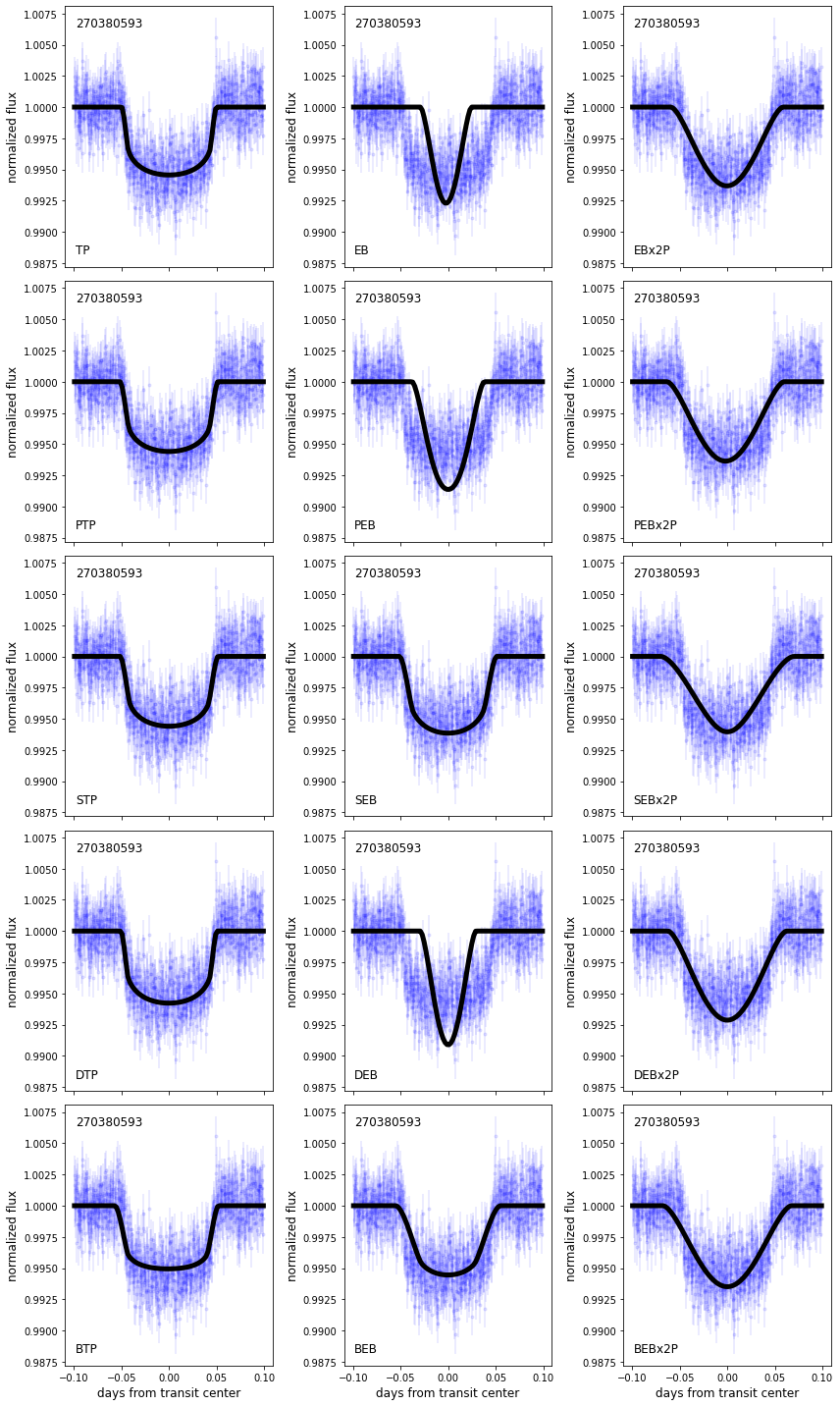
Now that that’s done, let’s check out a table of our results with the .probs attribute and calculate the false positive probability and nearby false positive probability using the .FPP and .NFPP attributes. We expect a scatter of a few percent in our probabilities, so don’t be alarmed if it’s slightly different with each run. We can also plot the transit fits of each scenario using the .plot_fits(time, flux_0, flux_err_0) method.

[7]:

df_results = target.probs
print("FPP =", np.round(target.FPP, 4))
print("NFPP =", np.round(target.NFPP, 4))
df_results

FPP = 0.0257
NFPP = 0.0

[7]:

	ID	scenario	M_s	R_s	P_orb	inc	ecc	w	R_p	M_EB	R_EB	prob
0	270380593	TP	0.811000	0.847380	3.836169	88.333097	0.113006	113.614711	6.247005	0.000000	0.000000	8.969353e-01
1	270380593	EB	0.811000	0.847380	3.836169	81.575924	0.248700	18.816670	0.000000	0.750206	0.780463	0.000000e+00
2	270380593	EBx2P	0.811000	0.847380	7.672338	86.732359	0.440551	272.710761	0.000000	0.802865	0.829755	2.788198e-42
3	270380593	PTP	0.811000	0.847380	3.836169	87.434474	0.013503	313.670909	6.689277	0.000000	0.000000	7.212812e-02
4	270380593	PEB	0.811000	0.847380	3.836169	85.730594	0.003117	273.231842	0.000000	0.100772	0.121108	8.221751e-281
5	270380593	PEBx2P	0.811000	0.847380	7.672338	86.700629	0.434983	285.997552	0.000000	0.775086	0.803671	1.607920e-37
6	270380593	STP	0.798209	0.825326	3.836169	88.325342	0.240162	166.823432	8.882569	0.000000	0.000000	2.565628e-02
7	270380593	SEB	0.645203	0.667594	3.836169	89.535783	0.046837	341.811599	0.000000	0.085054	0.100000	3.151474e-14
8	270380593	SEBx2P	0.208363	0.237596	7.672338	89.400395	0.475742	252.902277	0.000000	0.200939	0.230855	1.641204e-44
9	270380593	DTP	0.811000	0.847380	3.836169	88.067831	0.284716	8.442403	6.457548	0.000000	0.000000	5.280339e-03
10	270380593	DEB	0.811000	0.847380	3.836169	82.014739	0.086656	89.034830	0.000000	0.768497	0.797546	0.000000e+00
11	270380593	DEBx2P	0.811000	0.847380	7.672338	86.856205	0.474255	269.832690	0.000000	0.770544	0.799449	4.519202e-48
12	270380593	BTP	1.128000	1.551273	3.836169	83.008073	0.792758	8.566595	19.429841	0.000000	0.000000	4.979879e-13
13	270380593	BEB	0.705000	0.635519	3.836169	88.650061	0.179127	306.497063	0.000000	0.136785	0.167045	2.463958e-31
14	270380593	BEBx2P	0.970000	1.120520	7.672338	84.933593	0.000032	301.531167	0.000000	0.939502	0.991405	3.805488e-37

[8]:

target.plot_fits(time=time, flux_0=flux, flux_err_0=np.mean(flux_err))

If you plan to quote these results in a paper, you should run .calc_probs() several times and quote the mean and standard deviation of the FPP. This way, you can show that your result is not sensitive to the intrinsic scatter in the calculation.

We illustrate this below by calculating the FPP 20 times. We use the optional argument parallel to enable parallel light curve simulation, which makes the calculation ~5x faster. Enabling parallelization yields the same results as the non-parallel option, so you should feel free to set this argument to True at all times.

[11]:

%%time

FPPs = np.zeros(20)
for i in range(20):
    target.calc_probs(time=lc.time.value,
                      flux_0=lc.flux.value,
                      flux_err_0=np.mean(lc.flux_err.value),
                      P_orb=P_orb,
                      parallel=True,
                      verbose=0)
    FPPs[i] = target.FPP

meanFPP = np.round(np.mean(FPPs), 4)
stdvFPP = np.round(np.std(FPPs), 4)
print("FPP =", meanFPP, "+/-", stdvFPP)

...
...
...
...
...
...
FPP = 0.0432 +/- 0.0578
CPU times: user 19min 43s, sys: 1min 39s, total: 21min 23s
Wall time: 20min 9s

The FPP is favorable, but is not low enough to validate the planet.

Example #2#

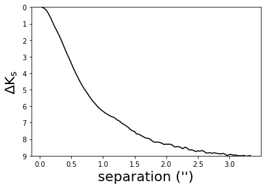
Next, let’s repeat this calculation while folding in follow up data. We’ll see how including a contrast curve of the target star changes these results and further constrains the FPP. Note that the contrast curve file should be a csv with no headers, where the first column is the angular separation (in arcseconds) and the second column is the \(\Delta\) mag.

[12]:

contrastcurve_file = "TOI465_01_contrastcurve.csv"
cc = pd.read_csv(contrastcurve_file, header=None)
sep, dmag = cc[0].values, cc[1].values

plt.plot(sep, dmag, 'k-');
plt.ylim(9,0);
plt.ylabel("$\\Delta K_s$", fontsize=20);
plt.xlabel("separation ('')", fontsize=20);

[13]:

%%time

FPPs = np.zeros(20)
for i in range(20):
    target.calc_probs(time=lc.time.value,
                      flux_0=lc.flux.value,
                      flux_err_0=np.mean(lc.flux_err.value),
                      P_orb=P_orb,
                      contrast_curve_file=contrastcurve_file,
                      parallel=True,
                      verbose=0)
    FPPs[i] = target.FPP

meanFPP = np.round(np.mean(FPPs), 4)
stdvFPP = np.round(np.std(FPPs), 4)
print("FPP =", meanFPP, "+/-", stdvFPP)

...
...
...
...
...
...
...
...
...
...
...
...
...
...
...
...
...
...
FPP = 0.0032 +/- 0.005
CPU times: user 18min 18s, sys: 1min 16s, total: 19min 34s
Wall time: 20min 24s

Folding in the follow up reduced the FPP to < 0.01! This is low enough to consider the planet validated.

Example #3#

Lastly, let’s apply the tool to TOI 411.02 (aka TIC 100990000.02), which was observed with a 2 minute cadence in sectors 3 and 4.

[14]:

ID = 100990000
sectors = np.array([3,4])
target = tr.target(ID=ID, sectors=sectors)

[15]:

ap_s3 = np.array([                            [185, 1320], [186, 1320],
                                 [184, 1319], [185, 1319], [186, 1319], [187, 1319],
                    [183, 1318], [184, 1318], [185, 1318], [186, 1318], [187, 1318],
                    [183, 1317], [184, 1317], [185, 1317], [186, 1317], [187, 1317],
                                 [184, 1316], [185, 1316], [186, 1316], [187, 1316]])

ap_s4 = np.array([  [414, 998], [415, 998], [416, 998],
                    [414, 997], [415, 997], [416, 997], [417, 997],
                    [414, 996], [415, 996], [416, 996], [417, 996],
                    [414, 995], [415, 995], [416, 995], [417, 995],
                    [414, 994], [415, 994], [416, 994], [417, 994],
                                            [416, 993]])

apertures = np.array([ap_s3, ap_s4])

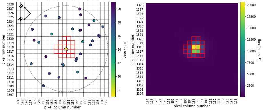
for i,(sector,aperture) in enumerate(zip(sectors,apertures)):
    print("Sector", sector)
    target.plot_field(sector=sector, ap_pixels=aperture)

target.stars

Sector 3

Sector 4

[15]:

	ID	Tmag	ra	dec	mass	rad	Teff	plx	sep (arcsec)	PA (E of N)
0	100990000	7.7570	54.819841	-42.762551	1.170000	1.116720	6161.0	15.899900	0.000	0.000
1	100990001	17.5993	54.793531	-42.764160	NaN	NaN	6245.0	0.492555	69.779	265.230
2	651027929	18.7320	54.795230	-42.771759	0.660000	0.537365	4205.0	-0.107290	73.003	242.987
3	100989999	18.1747	54.791855	-42.761727	NaN	NaN	NaN	NaN	74.028	272.289
4	100989997	16.6482	54.803113	-42.745878	0.501413	0.503408	3449.0	NaN	74.554	323.616
5	100989996	16.0327	54.801156	-42.745691	1.070000	1.198800	5910.0	0.298758	78.255	320.857
6	100990003	14.3572	54.808848	-42.784554	NaN	3.494880	5040.0	0.319435	84.367	200.136
7	100992258	13.2329	54.856880	-42.762261	NaN	7.990850	4760.0	0.260391	97.900	89.400
8	100990004	15.9458	54.838172	-42.786316	0.660000	0.596048	4218.0	1.477730	98.314	150.487
9	651027983	20.7092	54.833929	-42.736933	NaN	NaN	NaN	NaN	99.460	21.995
10	100990008	17.1068	54.827179	-42.791885	1.010000	0.638591	5668.0	0.351775	107.367	169.599
11	651027924	20.6024	54.826463	-42.792855	NaN	NaN	NaN	NaN	110.487	170.889
12	100990007	17.4834	54.794627	-42.789099	NaN	NaN	NaN	NaN	116.504	214.873
13	100989998	14.2672	54.774463	-42.753253	1.160000	1.209260	6137.0	0.715483	124.526	285.577
14	100990010	17.7780	54.797877	-42.794559	0.309075	0.328253	3401.0	1.974120	129.016	206.726
15	100992262	15.8841	54.861614	-42.742871	1.890000	1.825940	7908.0	0.001260	131.200	57.329
16	651027992	18.1822	54.790568	-42.731144	NaN	NaN	5601.0	-0.163846	137.015	325.601
17	651027993	18.8538	54.807099	-42.725453	NaN	NaN	3646.0	2.157550	137.738	345.839
18	100992250	17.7107	54.869454	-42.783607	0.399627	0.407237	3417.0	1.362360	151.442	120.051
19	651027921	20.1384	54.823442	-42.805121	NaN	NaN	NaN	0.448897	153.547	176.449
20	651027982	20.4606	54.870159	-42.740246	NaN	NaN	NaN	NaN	155.374	58.899
21	651027923	19.3605	54.797525	-42.804805	NaN	NaN	4749.0	0.307366	163.141	201.180
22	100990011	18.2129	54.795008	-42.805048	0.590000	0.425768	3847.0	0.867494	166.465	203.204
23	651027931	20.0574	54.756491	-42.755694	NaN	NaN	NaN	2.231890	169.256	278.365
24	651027920	20.4112	54.846882	-42.806245	NaN	NaN	NaN	-0.201713	172.762	155.581
25	100989992	16.5542	54.842338	-42.716863	1.020000	0.649991	5715.0	0.500855	174.904	19.890
26	651027482	18.4864	54.888120	-42.772374	0.620000	0.572985	3992.0	0.262623	183.882	101.111
27	100990014	14.5485	54.822924	-42.813591	1.060000	1.161500	5870.0	0.705178	183.922	177.463
28	651027986	18.9344	54.886834	-42.748117	NaN	NaN	4030.0	0.762538	184.552	73.669
29	651027919	20.0979	54.855863	-42.810432	NaN	NaN	NaN	0.802713	196.897	151.108
30	100990015	17.4240	54.803639	-42.816500	0.990000	0.666959	5606.0	0.194394	198.877	192.424
31	100989990	18.0093	54.797750	-42.709213	NaN	NaN	3883.0	1.127660	200.705	343.072

[16]:

target.calc_depths(tdepth=0.000166, all_ap_pixels=apertures)
target.stars

[16]:

	ID	Tmag	ra	dec	mass	rad	Teff	plx	sep (arcsec)	PA (E of N)	fluxratio	tdepth
0	100990000	7.7570	54.819841	-42.762551	1.170000	1.116720	6161.0	15.899900	0.000	0.000	9.999181e-01	0.000166
1	100990001	17.5993	54.793531	-42.764160	NaN	NaN	6245.0	0.492555	69.779	265.230	7.972274e-06	0.000000
2	651027929	18.7320	54.795230	-42.771759	0.660000	0.537365	4205.0	-0.107290	73.003	242.987	8.916198e-07	0.000000
3	100989999	18.1747	54.791855	-42.761727	NaN	NaN	NaN	NaN	74.028	272.289	3.097199e-06	0.000000
4	100989997	16.6482	54.803113	-42.745878	0.501413	0.503408	3449.0	NaN	74.554	323.616	1.950503e-05	0.000000
5	100989996	16.0327	54.801156	-42.745691	1.070000	1.198800	5910.0	0.298758	78.255	320.857	2.098939e-05	0.000000
6	100990003	14.3572	54.808848	-42.784554	NaN	3.494880	5040.0	0.319435	84.367	200.136	1.293266e-05	0.000000
7	100992258	13.2329	54.856880	-42.762261	NaN	7.990850	4760.0	0.260391	97.900	89.400	1.378523e-05	0.000000
8	100990004	15.9458	54.838172	-42.786316	0.660000	0.596048	4218.0	1.477730	98.314	150.487	2.638980e-06	0.000000
9	651027983	20.7092	54.833929	-42.736933	NaN	NaN	NaN	NaN	99.460	21.995	1.717102e-08	0.000000
10	100990008	17.1068	54.827179	-42.791885	1.010000	0.638591	5668.0	0.351775	107.367	169.599	5.900667e-08	0.000000
11	651027924	20.6024	54.826463	-42.792855	NaN	NaN	NaN	NaN	110.487	170.889	1.071358e-09	0.000000
12	100990007	17.4834	54.794627	-42.789099	NaN	NaN	NaN	NaN	116.504	214.873	1.378635e-10	0.000000
13	100989998	14.2672	54.774463	-42.753253	1.160000	1.209260	6137.0	0.715483	124.526	285.577	1.837653e-09	0.000000
14	100990010	17.7780	54.797877	-42.794559	0.309075	0.328253	3401.0	1.974120	129.016	206.726	3.512156e-12	0.000000
15	100992262	15.8841	54.861614	-42.742871	1.890000	1.825940	7908.0	0.001260	131.200	57.329	9.318788e-11	0.000000
16	651027992	18.1822	54.790568	-42.731144	NaN	NaN	5601.0	-0.163846	137.015	325.601	1.893848e-11	0.000000
17	651027993	18.8538	54.807099	-42.725453	NaN	NaN	3646.0	2.157550	137.738	345.839	7.346003e-12	0.000000
18	100992250	17.7107	54.869454	-42.783607	0.399627	0.407237	3417.0	1.362360	151.442	120.051	6.457540e-12	0.000000
19	651027921	20.1384	54.823442	-42.805121	NaN	NaN	NaN	0.448897	153.547	176.449	1.325042e-15	0.000000
20	651027982	20.4606	54.870159	-42.740246	NaN	NaN	NaN	NaN	155.374	58.899	1.010465e-16	0.000000
21	651027923	19.3605	54.797525	-42.804805	NaN	NaN	4749.0	0.307366	163.141	201.180	1.183616e-18	0.000000
22	100990011	18.2129	54.795008	-42.805048	0.590000	0.425768	3847.0	0.867494	166.465	203.204	6.155347e-19	0.000000
23	651027931	20.0574	54.756491	-42.755694	NaN	NaN	NaN	2.231890	169.256	278.365	3.622098e-19	0.000000
24	651027920	20.4112	54.846882	-42.806245	NaN	NaN	NaN	-0.201713	172.762	155.581	7.213192e-19	0.000000
25	100989992	16.5542	54.842338	-42.716863	1.020000	0.649991	5715.0	0.500855	174.904	19.890	2.632556e-17	0.000000
26	651027482	18.4864	54.888120	-42.772374	0.620000	0.572985	3992.0	0.262623	183.882	101.111	1.112206e-18	0.000000
27	100990014	14.5485	54.822924	-42.813591	1.060000	1.161500	5870.0	0.705178	183.922	177.463	1.800458e-19	0.000000
28	651027986	18.9344	54.886834	-42.748117	NaN	NaN	4030.0	0.762538	184.552	73.669	1.345936e-22	0.000000
29	651027919	20.0979	54.855863	-42.810432	NaN	NaN	NaN	0.802713	196.897	151.108	5.313263e-24	0.000000
30	100990015	17.4240	54.803639	-42.816500	0.990000	0.666959	5606.0	0.194394	198.877	192.424	1.544053e-25	0.000000
31	100989990	18.0093	54.797750	-42.709213	NaN	NaN	3883.0	1.127660	200.705	343.072	1.367531e-23	0.000000

[17]:

%%time

# read in the light curve
lc = pd.read_csv("TOI411_02_lightcurve.csv", header=None)
time, flux, flux_err = lc[0].values, lc[1].values, lc[2].values
P_orb = 4.040051

lc_binsize = (time.max()-time.min())/100
lc = TessLightCurve(time=time, flux=flux, flux_err=flux_err).bin(time_bin_size=lc_binsize)

target.calc_probs(time=lc.time.value, flux_0=lc.flux.value, flux_err_0=np.mean(lc.flux_err.value), P_orb=P_orb,
                  parallel=True)

TRILEGAL form submitted.
Calculating TP, EB, and EBx2P scenario probabilities for 100990000.
Calculating PTP, PEB, and PEBx2P scenario probabilities for 100990000.
Calculating STP, SEB, and SEBx2P scenario probabilities for 100990000.
Calculating DTP, DEB, and DEBx2P scenario probabilities for 100990000.
...
Calculating BTP, BEB, and BEBx2P scenario probabilities for 100990000.
CPU times: user 50.2 s, sys: 4.42 s, total: 54.6 s
Wall time: 1min 3s

[18]:

df_results = target.probs
print("FPP =", np.round(target.FPP, 4))
print("NFPP =", np.round(target.NFPP, 4))
df_results

FPP = 0.0399
NFPP = 0.0

[18]:

	ID	scenario	M_s	R_s	P_orb	inc	ecc	w	R_p	M_EB	R_EB	prob
0	100990000	TP	1.170000	1.116720	4.040051	87.430810	0.619036	329.591045	1.606318	0.000000	0.000000	7.506777e-01
1	100990000	EB	1.170000	1.116720	4.040051	82.582402	0.618804	306.214282	0.000000	1.075974	1.116720	1.139451e-58
2	100990000	EBx2P	1.170000	1.116720	8.080102	85.792644	0.828554	248.078683	0.000000	1.136131	1.116720	1.811696e-48
3	100990000	PTP	1.170000	1.116720	4.040051	87.424252	0.397792	323.801387	1.585492	0.000000	0.000000	1.188953e-01
4	100990000	PEB	1.170000	1.116720	4.040051	78.964877	0.282007	23.772130	0.000000	1.087470	1.116720	1.765332e-60
5	100990000	PEBx2P	1.170000	1.116720	8.080102	85.522643	0.598110	304.412358	0.000000	1.134997	1.116720	2.087916e-53
6	100990000	STP	1.060924	1.116720	4.040051	87.249296	0.341908	325.056354	2.677714	0.000000	0.000000	3.378508e-02
7	100990000	SEB	0.213924	0.242618	4.040051	88.345399	0.931711	249.880757	0.000000	0.042947	0.100000	5.009660e-18
8	100990000	SEBx2P	0.351836	0.361533	8.080102	88.270721	0.900819	254.730922	0.000000	0.345782	0.356475	4.586207e-15
9	100990000	DTP	1.170000	1.116720	4.040051	87.282509	0.368578	313.623482	1.567885	0.000000	0.000000	9.049978e-02
10	100990000	DEB	1.170000	1.116720	4.040051	79.895366	0.277093	12.269202	0.000000	0.940363	0.992628	3.327247e-61
11	100990000	DEBx2P	1.170000	1.116720	8.080102	85.574137	0.822941	245.756969	0.000000	1.124392	1.116720	3.731821e-52
12	100990000	BTP	1.034000	0.983545	4.040051	89.340025	0.553490	327.379648	18.977031	0.000000	0.000000	1.001123e-04
13	100990000	BEB	0.866000	1.283195	4.040051	88.984593	0.274950	354.593941	0.000000	0.303919	0.321197	5.996511e-03
14	100990000	BEBx2P	1.257000	1.427912	8.080102	85.359789	0.089682	302.623192	0.000000	1.255807	1.402719	4.546522e-05

[19]:

target.plot_fits(time=lc.time.value, flux_0=lc.flux.value, flux_err_0=np.mean(lc.flux_err.value))

TRICERATOPS

TESS example

Contents

TESS example#

Example #1#

Example #2#

Example #3#