Kepler example

This notebook walks through a few examples that show how to use TRICERATOPS. The examples below show:

1. How to apply TRICERATOPS on a star observed in a \(\textbf{single}\) \({\it Kepler}\) quarter \(\textbf{without}\) follow up data.

import numpy as np
import pandas as pd
import time
from lightkurve import KeplerLightCurve
import sys
import matplotlib.pyplot as plt
%matplotlib inline

import triceratops.triceratops as tr

import warnings
warnings.filterwarnings('ignore')

Let’s apply the tool on Kepler-10b (KIC 11904151), the first terrestrial planet discovered by Kepler (https://ui.adsabs.harvard.edu/abs/2011ApJ…729…27B/abstract).

Begin by defining the target star object with the target(ID, sectors) class. The arguments for this class are ID (the KIC ID of the star) and sectors (the quarters in which the star was observed). ID should be an integer and sectors should be a numpy array.

We’ll use quarter 3 for this example, although any combination of quarters would be valid.

ID = 11904151
sectors = np.array([3])
target = tr.target(ID=ID, sectors=sectors, mission="Kepler")

Next, let’s define the aperture used to extract the light curve, plot an image of the field, and display a table of nearby stars.

The aperture should be a 2D numpy array with the formal [[col#, row#], [col#, row#], [col#, row#], ...], where where each [col#, row#] is the column and row number of the pixel.

An image of the field can be plotted with the .plot_field(sector, ap_pixels) method. This method takes as optional arguments sector (the image sector you would like to plot) and ap_pixels (the aperture we just defined).

We can display a table of the stars in the image with the .stars attribute. This table contains the separation and position angle of each star from the target star, so that each can be identified in the plot. Note that the “ID” column lists the TIC ID of each star, not the KIC ID.

Note that the scale of a TESS pixel is about 20 arcseconds and a Kepler/K2 pixel is about 4.

ap = np.array([            [655, 247],
               [654, 246], [655, 246], [656, 246],
                           [655, 245]             ])

target.plot_field(sector=3, ap_pixels=ap)

target.stars

	ID	Tmag	Jmag	Hmag	Kmag	ra	dec	mass	rad	Teff	plx	sep (arcsec)	PA (E of N)
0	377780790	10.4767	9.889	9.563	9.496	285.679422	50.241306	1.017	1.089740	5706.0	5.361850	0.000	0.000
1	1717218059	17.8806	NaN	NaN	NaN	285.680619	50.245790	1.070	0.809877	5895.0	-0.111711	16.375	9.693
2	1717218056	20.0671	NaN	NaN	NaN	285.677382	50.248546	NaN	NaN	NaN	0.879011	26.486	349.788
3	1717218060	17.4027	NaN	NaN	NaN	285.680220	50.249945	1.030	1.055070	5771.0	-0.004017	31.154	3.380
4	377780779	15.8564	14.727	14.117	14.075	285.685892	50.249906	0.700	0.804521	4467.0	0.999995	34.356	25.690
5	1717218057	18.4788	NaN	NaN	NaN	285.682207	50.251926	NaN	NaN	4923.0	0.325102	38.767	9.518

We can now determine which stars in the aperture are bright enough to produce the observed transit. The transit for this TOI has a depth of ~190 ppm. We’ll use the .calc_depths(tdepth, all_ap_pixels) method to do this. This method takes as arguments tdepth (the transit depth of the candidate) and all_ap_pixels (a numpy array of all apertures). After doing this, the .stars table includes the flux ratio contributed by each star in the aperture and the transit depth each star would have if it were the host of the signal.

apertures = np.array([ap])
target.calc_depths(tdepth=0.00019, all_ap_pixels=apertures)
target.stars

	ID	Tmag	Jmag	Hmag	Kmag	ra	dec	mass	rad	Teff	plx	sep (arcsec)	PA (E of N)	fluxratio	tdepth
0	377780790	10.4767	9.889	9.563	9.496	285.679422	50.241306	1.017	1.089740	5706.0	5.361850	0.000	0.000	9.999993e-01	0.00019
1	1717218059	17.8806	NaN	NaN	NaN	285.680619	50.245790	1.070	0.809877	5895.0	-0.111711	16.375	9.693	6.626514e-07	0.00000
2	1717218056	20.0671	NaN	NaN	NaN	285.677382	50.248546	NaN	NaN	NaN	0.879011	26.486	349.788	1.308192e-14	0.00000
3	1717218060	17.4027	NaN	NaN	NaN	285.680220	50.249945	1.030	1.055070	5771.0	-0.004017	31.154	3.380	4.187665e-19	0.00000
4	377780779	15.8564	14.727	14.117	14.075	285.685892	50.249906	0.700	0.804521	4467.0	0.999995	34.356	25.690	2.692696e-22	0.00000
5	1717218057	18.4788	NaN	NaN	NaN	285.682207	50.251926	NaN	NaN	4923.0	0.325102	38.767	9.518	4.131923e-30	0.00000

After doing this, we can calculate the probability of each scenario using the .calc_prob(time, flux_0, flux_err_0, P_orb) method, which requires as arguments time (times from phase-folded light curve in units of days from transit center), flux_0 (normalized flux from phase-folded light curve), flux_err_0 (flux error values of the target’s phase-folded light curve), and P_orb (orbital period of the TOI in days).

# read in the light curve
lc = pd.read_csv("Kepler10b_lightcurve.csv", header=None)
time, flux, flux_err = lc[0].values, lc[1].values, lc[2].values
P_orb = 0.837

mask = ~np.isnan(flux)
lc = KeplerLightCurve(time=time[mask], flux=flux[mask], flux_err=flux_err[mask])

lc.plot();

%%time

target.calc_probs(time=lc.time.value, flux_0=lc.flux.value, flux_err_0=np.mean(lc.flux_err.value),
                  P_orb=P_orb, parallel=True)

Calculating TP, EB, and EBx2P scenario probabilities for 377780790.
Calculating PTP, PEB, and PEBx2P scenario probabilities for 377780790.
Calculating STP, SEB, and SEBx2P scenario probabilities for 377780790.
Calculating DTP, DEB, and DEBx2P scenario probabilities for 377780790.
Calculating BTP, BEB, and BEBx2P scenario probabilities for 377780790.
CPU times: user 4min 40s, sys: 50.1 s, total: 5min 30s
Wall time: 3min 47s

Now that that’s done, let’s check out a table of our results with the .probs attribute and calculate the false positive probability and nearby false positive probability using the .FPP and .NFPP attributes. We expect a scatter of a few percent in our probabilities, so don’t be alarmed if it’s slightly different with each run. We can also plot the transit fits of each scenario using the .plot_fits(time, flux_0, flux_err_0) method.

df_results = target.probs
print("FPP =", target.FPP)
print("NFPP =", target.NFPP)
df_results

FPP = 8.359147213754525e-06
NFPP = 0.0

	ID	scenario	M_s	R_s	P_orb	inc	ecc	w	R_p	M_EB	R_EB	prob
0	377780790	TP	1.017000	1.089740	0.837	81.941887	0.137458	301.973062	1.530357	0.000000	0.000000	9.986258e-01
1	377780790	EB	1.017000	1.089740	0.837	62.306030	0.125414	155.004503	0.000000	0.902493	0.940614	0.000000e+00
2	377780790	EBx2P	1.017000	1.089740	1.674	79.804803	0.593447	271.445956	0.000000	0.969306	1.034376	0.000000e+00
3	377780790	PTP	1.017000	1.089740	0.837	83.379944	0.099257	339.859299	2.055697	0.000000	0.000000	1.322033e-03
4	377780790	PEB	1.017000	1.089740	0.837	60.451731	0.114222	122.593120	0.000000	0.953240	1.011065	0.000000e+00
5	377780790	PEBx2P	1.017000	1.089740	1.674	79.770569	0.620781	266.299544	0.000000	0.999198	1.078092	0.000000e+00
6	377780790	STP	0.951171	1.008085	0.837	83.692681	0.237393	326.519230	2.119661	0.000000	0.000000	8.359147e-06
7	377780790	SEB	0.109903	0.133778	0.837	73.517626	0.861199	10.740936	0.000000	0.017933	0.100000	0.000000e+00
8	377780790	SEBx2P	0.193797	0.224327	1.674	87.099013	0.827427	260.175941	0.000000	0.185594	0.216743	0.000000e+00
9	377780790	DTP	1.017000	1.089740	0.837	87.448863	0.505783	350.343154	1.475852	0.000000	0.000000	4.379518e-05
10	377780790	DEB	1.017000	1.089740	0.837	64.745292	0.250926	205.266064	0.000000	0.953028	1.010759	0.000000e+00
11	377780790	DEBx2P	1.017000	1.089740	1.674	79.095540	0.508872	274.831562	0.000000	0.987414	1.060850	0.000000e+00
12	377780790	BTP	1.002000	1.003385	0.837	85.831615	0.295998	200.494018	14.884591	0.000000	0.000000	3.686393e-152
13	377780790	BEB	0.979000	0.920291	0.837	89.490265	0.477375	331.736262	0.000000	0.130606	0.159874	0.000000e+00
14	377780790	BEBx2P	1.252000	1.334553	1.674	74.255047	0.001115	357.936948	0.000000	1.250441	1.334553	0.000000e+00

target.plot_fits(time=lc.time.value, flux_0=lc.flux.value, flux_err_0=np.mean(lc.flux_err.value))

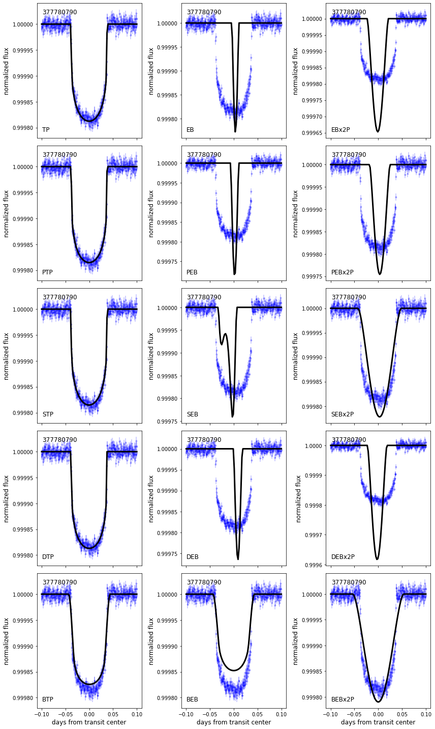
TRICERATOPS predicts that this planet candidate is a bona fide planet with a radius of ~1.5 \(R_\oplus\), which isn’t too far off from the radius reported in the literature. With this FPP, the planet would be considered validated.